

POST
Handy Excel Shortcuts for Digital PRs
Excel, Google Sheets and digital PR go together, hand in hand. There’s a high likelihood that you will have to deal with a spreadsheet of some kind during your first week in this industry, and your interaction with them will only increase as you move through your career. So, let’s have a look at some Excel shortcuts for digital PRs that will save you time and impress your colleagues.
The difference between Excel and Google Sheets formulas
Google Sheets is great for collaborating in real-time as more than one person can edit the document at the same time, whilst Excel has long been the preferred application for those who have an Office 365 account - with over 750 million users worldwide, it is a clear favourite.
Although Excel and Google Sheets have the same purpose, most people do have a preference. However, it’s also handy to know specific shortcuts and formulas that work on each just in case you’re required to work on the one you don’t use as often.
In terms of standard functions and formulas, the two applications are quite similar with SUM, MIN, COUNT, MAX and AVERAGE. You can either manually type the formula into the result cell or select it and choose from the menu under ‘Function’.

Let’s start with the basics
Some shortcuts are a quicker and easier way to carry out a process. Once you get to grips with these, you can use them alongside the trickier formulas to help with data collection and organisation.
Here are a few keyboard shortcuts, if you’re using an Apple product, the control key is usually replaced with command (⌘):
-
F2 - Use this to edit the contents in a cell (it is much quicker than double-clicking).
-
Ctrl + arrow keys - This allows you to navigate data very quickly.
-
Ctrl + Shift + arrow keys - This will give you the chance to highlight relevant cells quickly.
-
Ctrl + R - You can drag a formula across columns (used in conjunction with Ctrl + shift + arrow keys).
-
Ctrl + D - You can drag a formula across rows (used in conjunction with Ctrl + shift + arrow keys).
-
Ctrl + A - This selects all cells in a table.
-
Ctrl + Click - This allows you to select multiple cells that are not next to each other. Just hold down the control key and select all the cells you want.
These shortcuts will help you navigate your spreadsheets as well as populate the cells. You may also be interested in learning shortcuts to format on Excel and Google Sheets:
-
Bold - Ctrl + B
-
Italic - Ctrl + I
- Underline - Ctrl + U
Excel shortcuts for data organisation
Once you have all of your data transferred to your Excel or Google sheet, you can start to organise it. This allows you to draw conclusions from your data, showing rankings or display percentage changes clearly.
One of the most common ways to organise data is to use the Sort function in Excel. You just need to highlight the data you want to organise, right-click and choose ‘Sort’. You can then choose from:
-
Smallest to largest
-
Largest to smallest
-
Put selected cell colour on top
-
Put selected font colour on top
-
Put selected formatting icon on top
Having a few shortcuts and formulas like these will help you organise your data and save you time to better plan your day as a digital PR.
Handy formulas to streamline your workflow
Working as a digital PR, or in a digital PR company, can be tricky business, so anything that will help you achieve something quicker will help to streamline your workflow and allow you to focus on other aspects of your role. Here are some handy formulas digital PRs often use day-to-day:
SUM
Perhaps the most used function in Excel, this will add together the values from a selection of cells to easily see the highest and lowest. Input the following into the result cell:
=SUM(cell number 1, cell number 2, etc.)
Some examples:
=SUM(A1:H1) - This will sum the values of a row and display them in the result cell.
=SUM(A1:A10) - Instead of a row, this will sum the values of a column
=SUM(A1:A5, A7, A10:A17) - This is great if you want to skip a few cells but don’t want more than one sum. This example skips cells A6, A8 and A9.
You can also find the SUM function on your toolbar.
COUNT
The COUNT function will count all numerical values in your chosen selection. You can type in:
=COUNT(cell 1, cell 2, etc.)
Some examples:
COUNT(A:A) - This will count all of the numerical values in the A column.
COUNT(A1:E1) - Much like the previous one, but this will count rows instead.
COUNTA
Like the COUNT function, COUNTA counts all cells within your selected range, but the cells do not need numerical values. This function is good if you need to count dates, times, text or errors.
=COUNTA(cell 1, cell 2, etc.)
Some examples:
COUNTA(A1:A10) - This will count rows 1 to 10 in column A.
COUNTA(A1:E1) - This will count the cells in this row.
AVERAGE
This is great if you want to quickly work out the average of a few cells or calculate the average result from a list. If you want to do it manually rather than use the Autosum feature, type in:
=AVERAGE(cell number 1, cell number 2, etc.)
An example:
=AVERAGE(A1:A10) - Will calculate an average using all values from this range.
MIN and MAX
The MIN and MAX formula will find the minimum and maximum numbers in a selection of cells.
=MIN(cell number 1, cell number 2, etc.)
=MAX (cell number 1, cell number 2, etc.)
Some examples:
=MIN(A1:B10) - This will find the minimum number out of columns A and B, from row 1 to 11.
=MAX(A1:B10) - This will find the maximum number out of columns A and B, from row 1 to 11.
IF
The IF formula is when you want to fill the result cell with content that depends on the contents of other cells - it will only populate the cell if a condition has been met. This is where you can start getting clever with your data organisation to embed other formulas or functions within the IF formula.
=IF(condition is met, value if true, value if false)
Some examples:
=IF(A1>70, “TRUE”, “FALSE’”) - If the contents of A1 is greater than 70, then TRUE will appear in the result box. If it is not, then FALSE will appear.
=IF(AVERAGE(A1:A5) > AVERAGE(B1:B5), AVERAGE(A1:A5), AVERAGE(B1:B5)) - This is a complex variant of this formula that involves a few processes. First, it will calculate the average of cells A1 to A5, as well as B1 to B5 before comparing them. If the average of A1 to A5 is larger than B1 to B5, the result cell will be populated with this average. However, if it is not, it will be filled with an average of B1 to B5.
You can practice this with many other functions such as SUM and MAX/MIN.
TRIM
This is a handy way to eliminate blank spaces to make sure your results are accurate. However, this can only work within a single cell rather than a larger selection.
=TRIM(cell)
An example:
TRIM(A1) – This will remove all empty spaces in A1.
Conditional formatting
Conditional formatting is a great way to save time and add some visual elements to your spreadsheet on Excel. There are a few different things you can do with conditional formatting. Some will take some time to get to grips with, but here is an outline of the areas most used by digital PRs:
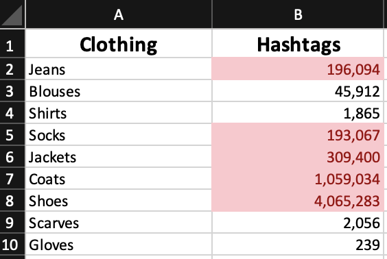
Highlight specific cells
This will help you to pinpoint specific values to help you draw conclusions or group together similar results. You can choose whether to highlight cells greater than or less than a certain value, between two values, equal to a number, containing specific words or numbers, after a certain date or any duplicates.
Here is an example where only cells with a value greater than 1,000 have been highlighted:
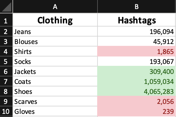
Top/bottom rules
This will allow you to find the top 10 (or any other number) as well as the bottom values. This type of formatting is beneficial if you’re looking at creating a campaign based on rankings.
You could format the cells in the top 10 a light green and the bottom 10 in red to make the data easily digestible. Here is an example where the top and bottom three have been formatted:
Data bars
To further illustrate your data, you can add data bars. These mean you can get a quick visual of your findings without looking at the individual numbers. Here is an example of a table with data bars:
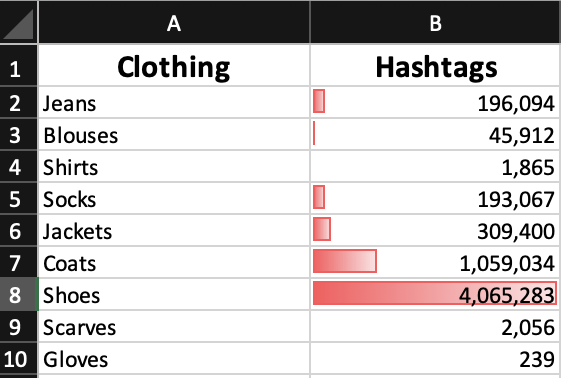
You can choose what colour you want the bars and whether you want them with a gradient effect or solid colour for further personalisation.
Colour scales
The colour scale conditional formatting is like the data bars in the way that it adds a visual aspect to your spreadsheet. It will show the ranking of your results in colour. In this example, green means the top values and red means the bottom:
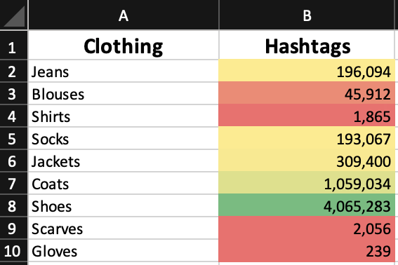
At a glance, you can easily see where in the ranking each item falls.
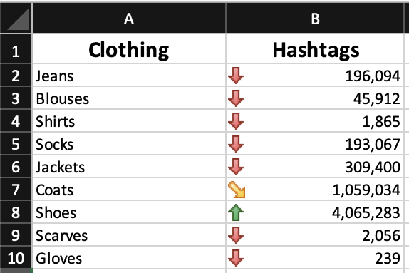
Icon sets
Icon Sets conditional formatting will add the icons of your choice to the data in order to help the understanding. It combines colours and shapes to show whether something is high up in the rankings or near the bottom. This is very helpful if you’re looking at percentage increase or decrease too.
Here is an example with green, red and yellow directional arrows:
These are just a few simple examples to get you started with conditional formatting. However, you will soon find that the more you work with this, the easier it will become and the more adventurous you will be.
 Resources to help digital PRs
 Organising your day as a digital PR
 Useful Digital PR tools
 The best data sources to use